A library is not a service: what it takes to put an LLM information extractor behind real traffic


In part one we went looking for the best way to pull four fields out of an NDA, and the benchmark handed back a clear winner: single-pass extraction with Gemini 3 Flash, scoring 91.5% F1 at ~$0.007 per document and under ten seconds of latency, past the pre-LLM baseline and matching the agentic strategy on accuracy at half its cost and latency.
That’s a satisfying place to end a benchmark. But a useless place to end a project.
A winning configuration is just a benchmark result, and the enterprise problem we opened part one with (people reading documents and typing the same handful of fields into a system of record) isn’t solved by a result. It’s solved by a service: something a system can hand a document to and get structured data back from, reliably, on a Tuesday morning when hundreds of documents arrive at once.
A library is not a service, and closing that gap is its own engineering problem, one the benchmark never had to think about. The library (agentic-kie) leaves four questions unanswered that a production system has no choice but to solve:
- How do you let a client hand you a document of any size, when the front door has a payload limit?
- How do you decouple the caller from a slow LLM call so nobody sits and waits ten seconds for a response?
- How do you make extraction retryable when it fails partway, without forcing the document to be uploaded again?
- How do you fit heavy LLM dependencies into a runtime that’s supposed to scale to zero?
Answer those four and a document becomes a structured record. That record then owes two audiences: the system that triggered the upload, which needs to know the moment its result is ready, and the team that owns extraction quality, which needs every result kept as a queryable dataset it can evaluate the live system against, sample failures from, and build fine-tuning sets out of.
The rest of this post is that architecture, the decisions that shaped it, and the load tests that put it under real arrival pressure. Since the pipeline runs both strategies behind one contract, those tests settle something part one couldn’t: whether agency ever earns its cost under load.
Where the infrastructure lives
The deployment layer is its own repository: agentic-kie-deploy. Everything in this post (the Terraform modules, the Lambda handlers, the load-testing harness, and the ADRs that justify each choice) is there and auditable; where a decision warrants more explanation than fits here, I link the relevant ADR.
The shape of the solution
The whole system is asynchronous and event-driven: no caller ever waits on an extraction, and nothing downstream is ever called directly, each stage just reacting to what the one before it produced.
From the outside, a caller touches only the front door and the back door:
- A caller asks for an upload slot and gets back a document ID and a short-lived URL.
- The caller uploads the document straight to that URL.
- The caller reads the structured result from an address it already knew at step one, or gets pinged the moment it lands.
An internal service with a small contract
This isn’t a public API. A deployment serves a known set of in-account callers, and it does one job: one document type, one result schema. That single schema is the design, not a limitation: it’s a template, deployed once per team, so a dozen diverging extraction needs run as a dozen small services rather than one shared platform routing them all.
The end-to-end pipeline
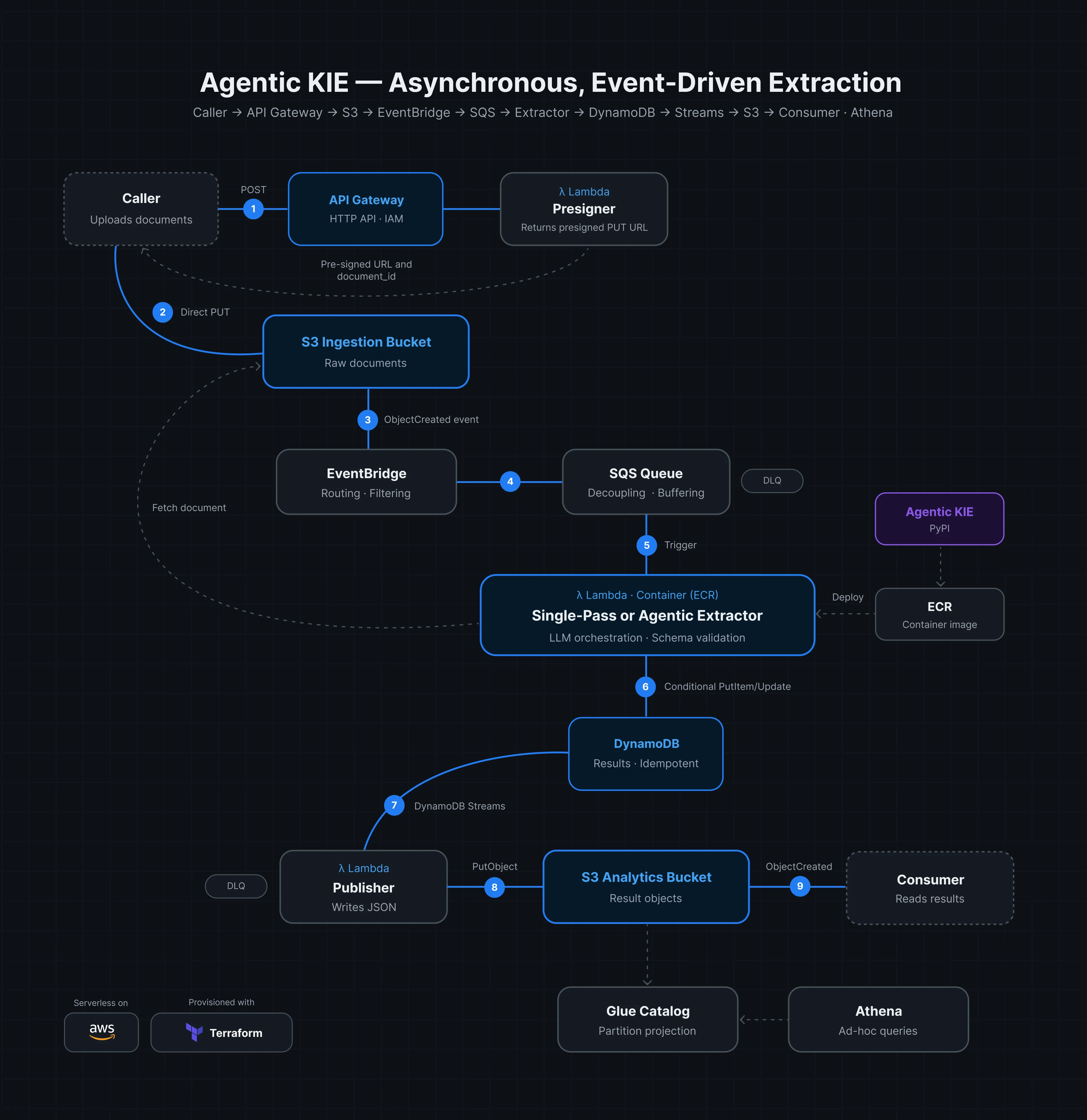
A document moves through it like this: the slot request hits a small presigner function, which mints an ID and returns a pre-signed upload URL. The upload lands directly in an S3 bucket, which emits an event; EventBridge routes it onto an SQS queue, which feeds the extractor, the container that runs agentic-kie.
The extractor writes its answer to a DynamoDB table; that write fans out through a stream to a publisher function, which drops the final result as JSON into a second S3 bucket at the address the caller learned in step one. A query layer (Glue and Athena) sits over those results for later analysis.
The DevOps strategy is part of the design
The entire stack is Terraform from end to end, and it ships itself: merges to develop and main deploy to staging and prod through CI, authenticating to AWS with short-lived OIDC tokens rather than stored keys. The environment model and deployment roles are documented in CONTRIBUTING.md.
Design, decision by decision
The architecture diagram is the what. What follows is the why: the rationale behind the most consequential design decisions.
The front door is a handshake
The naive design routes the document through an API: the caller POSTs the PDF, the server takes it, and passes it on. That’s a pipe, and it’s the wrong shape three times over:
- Every byte is proxied through your own compute, so you pay to move data you never needed to hold.
- Managed gateways cap request bodies, so a large document is rejected before extraction begins.
- They time out in seconds, long before a slow LLM call finishes.
So the front door does not carry the document. It carries a handshake: the presigner mints a document_id and returns a pre-signed URL, a time-limited permission slip to write a single object straight to S3. The caller uploads directly to storage, bypassing the API entirely.
The ID exists before the document does
The document_id is created at slot-request time, not after extraction. It names the storage location, it becomes the key the result is written under, and, because the caller learns it before uploading, it hands the caller the result’s future address in advance. The full lifecycle is in ADR-0006.
The same handshake is also its own security model: the slot request rides the caller’s existing cloud identity, so there are no API keys to rotate. The URL it returns is a bearer capability (anyone holding it can write to that one address), which is exactly why it expires within minutes: the expiry bounds what a leaked link is worth, to a few minutes of write access to a single key.
The handshake only fixes how the document gets in. The timeout, the caller left waiting on a slow LLM call, is not a front-door problem; it’s where the next section picks up.
The slow part is decoupled
The LLM call takes the better part of ten seconds, and sometimes much more. If the caller had to wait for it, the whole system would be only as fast and as available as its slowest extraction. So the caller doesn’t wait: the upload returns immediately, and the slow work happens on its own.
When the upload lands, S3 emits an event, and that event, not the caller, drives the rest of the pipeline. A queue sits between the upload and the extractor and acts as a shock absorber: when a batch of documents arrives at once, they pile up and drain at whatever rate the extractor can sustain. A synchronous pipe would start rejecting or timing out the moment traffic exceeded capacity; a queue just gets deeper, then drains.
The queue is a deliberate cost guardrail, not just a buffer
The extractor’s concurrency is capped on purpose: infinite scaling of an LLM call means an unbounded bill. The queue holds the burst the cap won’t let the extractor swallow at once. The two halves of that decision live in separate records: the queue intentionally doesn’t constrain fan-out (ADR-0005), and the cap that bounds it lives next to the extractor (ADR-0009).
Every attempt is retryable
Extraction will eventually fail: a transient provider error, a timeout, a rate limit. Two things have to be true when it does. A failed extraction must be retryable without re-uploading the document, and a retry must never corrupt a result that already succeeded.
The first falls out of the queue. A message that fails processing isn’t lost: it becomes visible again and is retried, a fixed number of times, against the document still sitting in storage. The caller does nothing. If every retry is exhausted, the message lands in a dead-letter queue: quarantine for poison documents, so one bad file can’t drain budget forever.
The second is subtler: at-least-once delivery means the same document can reach the extractor twice. The fix is idempotency: the extractor claims a document with a conditional write before doing any work, and writes its terminal result only if the row is still in the state it expects. A redelivered message that finds the work already done is a no-op.
One edge is left to a human on purpose. A worker that dies mid-extraction leaves its claim standing, and a redelivered message backs off rather than seizing it: the system can’t tell a dead claimant from a slow one, and won’t risk paying for the same extraction twice. Those retries exhaust into the dead-letter queue, where recovery is an operator’s decision.
Heavy where it has to be
The dependencies that make extraction work (the LLM client, the document parser, the model SDKs) don’t fit Lambda’s zipped package limits, and a cold runtime takes seconds to load them. The mistake would be to let that weight spread; instead it’s confined to the one function that runs the model.
The extractor ships as a container image from a private registry, large enough to hold everything the model call needs. Every other function stays light: the presigner that mints the upload slot and the publisher that writes the result are a handful of lines with no dependencies at all, thin zips that start instantly.
And that one heavy function still scales to zero, thanks to the decoupling from the section before. An image that size has a multi-second cold start: unacceptable on a synchronous front door, unnoticed behind a queue, where a few seconds on the first document of a burst is a delay nobody is waiting on. The extractor pays for no idle capacity and wakes only when documents arrive.
Provisioned concurrency buys nothing here
Provisioned concurrency would erase the multi-second cold start, but it bills for warm capacity around the clock: paying to scale to zero, then paying again not to. For a queue-driven consumer no caller is waiting on, it’s left off. The image’s size, digest pinning for deterministic rollback, and the registry it ships from are in ADR-0008; the function’s sizing and cold-start posture are in ADR-0009.
Where do results land?
A result needs to reach whoever asked for it. The obvious design is a status endpoint the caller polls, but polling is wasteful, adds latency, and quietly makes the result a caller’s problem to chase. A service should spend its own complexity to buy its consumers simplicity, not the reverse.
Instead, the result is written as a JSON object to a known S3 address: the one derived from the document_id the caller already holds. Consuming it is cheap: read that address directly, or subscribe to the bucket and get notified the instant the object appears.
The object itself is the extracted fields wrapped in just enough metadata to make it auditable:
{
  "document_id": "0190c3b2-7f4e-7a21-9c3d-1f2e3a4b5c6d",
  "status": "succeeded",
  "extracted_fields": {
    "effective_date": "2019-03-14",
    "jurisdiction": "Delaware",
    "party": [{ "name": "Nike_Inc." }, { "name": "Acme_LLC" }],
    "term": "2_years"
  },
  "model_version": "gemini-3-flash-preview",
  "token_usage": { "input": 8123, "output": 142 },
  "processing_ms": 8299
}
There's no 'in progress' object
A result object exists only for a terminal outcome: success or failure. A document still in flight simply has no object yet: “is it done yet?” is a question the storage layer answers by the file’s existence alone. Why S3 instead of an API is argued in ADR-0011.
The results are also a dataset
The dataset costs almost nothing to expose, because the result objects the system already writes are the dataset. AWS Glue crawls the JSON objects and registers a schema over them, so a folder of files becomes a catalogued table; Athena then reads that table straight from S3 with plain SQL. Nothing is copied or reshaped: the same object that delivers a result is the row a query returns.
The team that tunes extraction can then sample the failures, measure field-level accuracy over real traffic, and build a fine-tuning set out of documents the system has actually processed.
Part one evaluated the library once, on eighty-three documents from a frozen test partition. Production hands it a stream of real documents that never stops arriving, every one of them a case the next evaluation can use.
Two planes of observability
A production extraction service raises two very different questions that don’t belong in the same place.
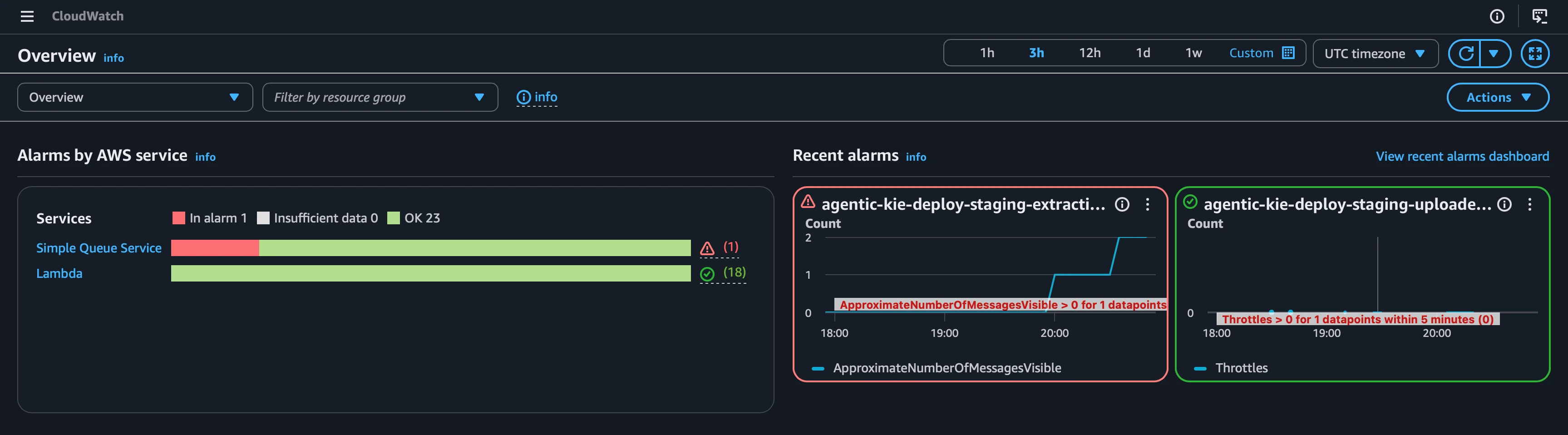
One is operational: did the function run, did it error, is the dead-letter queue filling, is the cap throttling? That’s minute-to-minute, and it lives in cloud metrics and alarms.
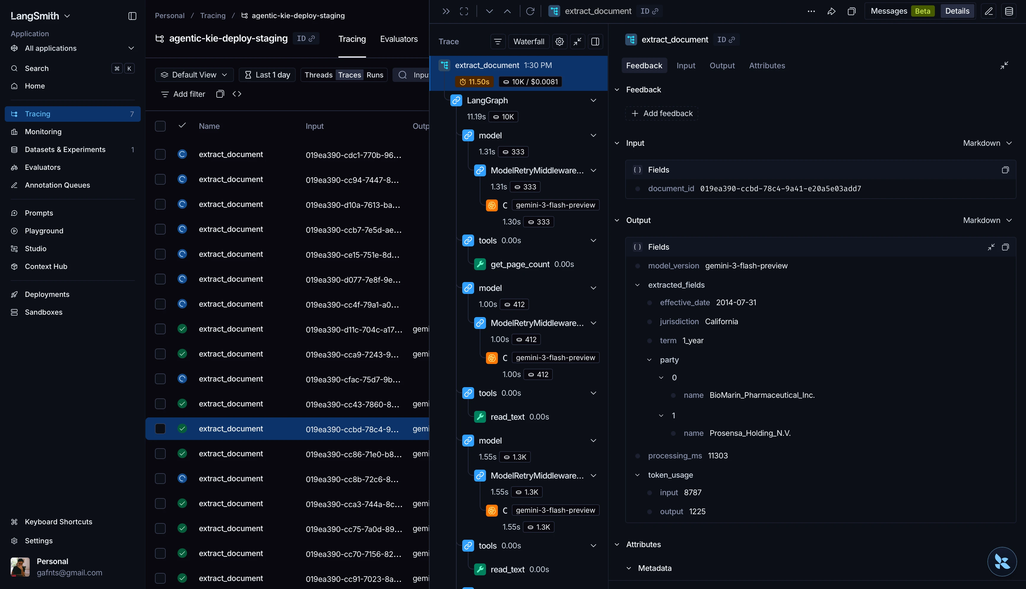
The other is model telemetry: what did the model see, how many tokens did it burn, did the output validate against the schema? That’s the question you ask over weeks of prompt iteration, and it lives in a purpose-built LLM-tracing tool.
LangSmith is fine here, not in production
The model backend shown above is a hosted SaaS: prompts and completions leave AWS and live at the vendor’s API for its retention window. That’s an acceptable trade at portfolio scale; it stops being acceptable once real documents arrive, on two triggers: data privacy, and spend. The switch is cheap (LangSmith’s data is OTel-compatible, so moving is a config change), though the destination, a self-hosted store like Langfuse, is an always-on service with its own compute and upkeep. When to move is in ADR-0009.
The two planes share exactly one thing: the document_id that correlates a trace to an invocation. Keeping them separate lets each question get its own answer at its own cadence.
Does it hold under load?
Every claim so far (buffering instead of failing, draining instead of choking, capping the bill) is a hypothesis until traffic proves it. So, in the spirit of part one’s benchmark, the pipeline gets the same treatment: write the predictions down first, then run real documents through the real system and grade what happened.
The question a load test answers here:
Does the system degrade gracefully (buffer and drain) rather than fail (error and dead-letter) under a realistic arrival pattern?
A calm moment, a hard spike
The two scenarios mark the edges of realistic operation rather than pushing the system until it snaps; both run the same 200 real NDAs (sampled from the Kleister train partition) through the live system end to end.
Two scenarios: a calm moment and a hard spike
Both push the same 200 real NDAs through the live system end to end
| Scenario | What it is | What it characterizes |
|---|---|---|
| Sustained | 200 documents at a steady rate | The calm, normal moment (the queue never builds) |
| Burst | 200 documents dumped as fast as the client can upload | The real stressor (the queue fills instantly) |
The sustained run is boring by design: uneventful is the result. The burst is where the architecture proves itself.
The queue absorbs, the cap holds, the backlog drains
Here’s what 200 documents arriving at once did to the single-pass pipeline: the queue spikes to nearly 200, then drains cleanly to zero in under four minutes while extractor concurrency sits flat at its cap of 10 (saturated, never exceeded).
The queue absorbs the spike, the cap paces the drain
Single-pass burst: 200 documents arriving at once, reconstructed from per-document queue-wait timings
That curve is reconstructed from per-document timings. The SQS console tells the same story in its own metrics: messages-visible spikes and drains to zero, and the oldest message ages to ~2.8 minutes before the backlog clears.
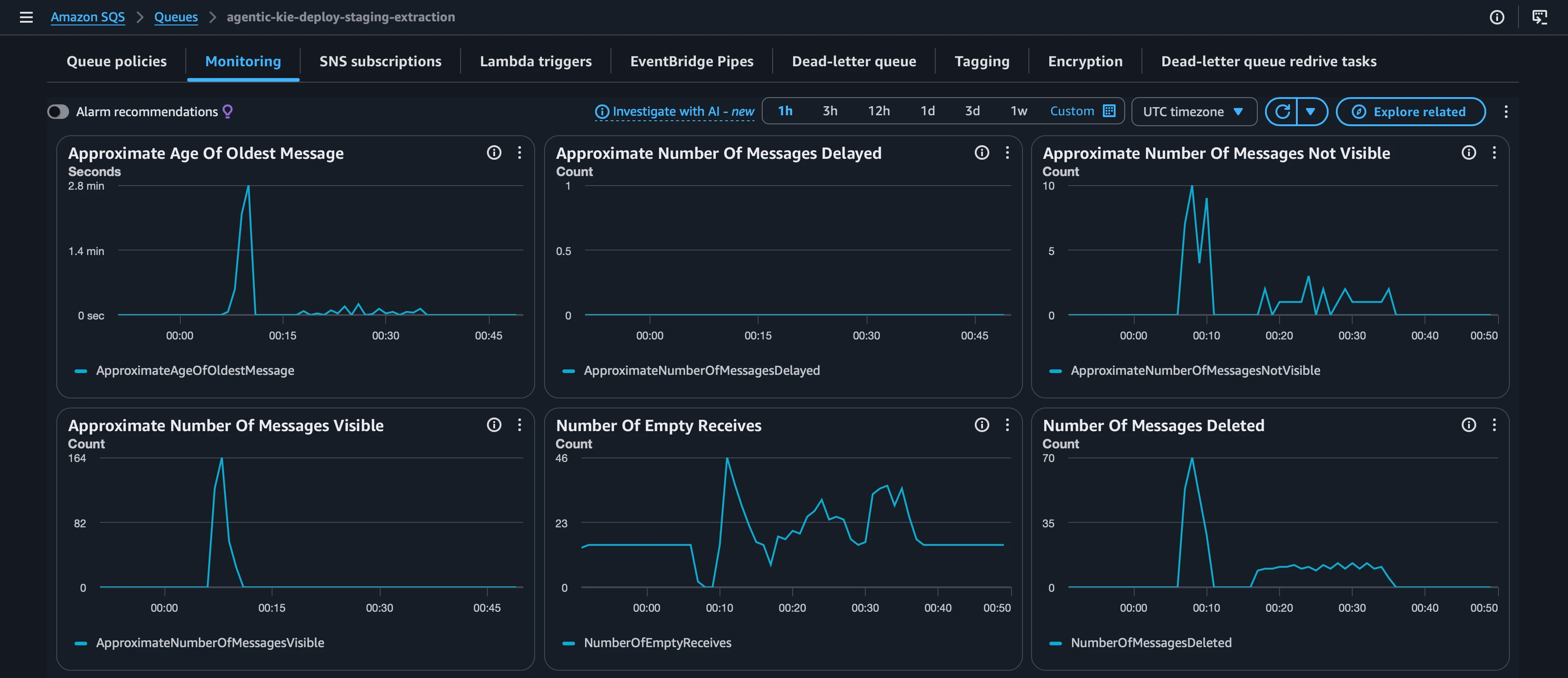
Behind that console view sits a scorecard of predictions, registered before the run, every one landed:
What happens when 200 documents arrive all at once?
Every prediction registered before the run, graded against the single-pass pipeline
| Metric | Result | The prediction it tested |
|---|---|---|
| Documents succeeded | 200 / 200 | Correctness: no failures, dead-letter queue empty |
| Queue peak depth | 192 | The shock absorber fills near-instantly |
| Oldest-message age | 167s (vs. 720s limit) | Drains before any message times out into a redelivery |
| Concurrency | Pinned at cap of 10, 0 throttles | The cost guardrail holds; the queue paces the work |
| Drain time | ~3.8 min | The backlog clears in minutes |
| Alarms fired | None | The operational plane stays quiet on a healthy run |
Every prediction landed, without a single throttle and without an alarm in this run: graceful degradation, measured rather than asserted.
That clean drain isn’t luck; it’s the one constraint every saturated queue obeys. Little’s Law says the average number of items in a system equals the rate they arrive times the time each one spends inside:
Point it at the extractor pool and it collapses. Under a burst the pool is pinned at its concurrency cap, so the work in flight is fixed at , and each document holds a worker for its service time . Rearranged, the rate the pool clears work is:
Cap over service time: not the arrival rate, not the burst size, not how deep the backlog gets. At a cap of 10 and the benchmark’s ~10s extraction that’s ~60 documents a minute; the run cleared 200 in 3.8 minutes, about 52 a minute, the gap being real-world overhead a benchmark never carries: the first document’s cold start, the publish hop.
The same law defuses the one number that looks alarming. The last documents in the burst came back at ~178s at the 90th percentile, against ~10s of actual extraction. That gap isn’t a bottleneck; it’s queue wait, the time a document spent in line. A burst of documents draining at empties in roughly , and the tail of the line waits nearly that whole time before its own extraction even starts. The 178s is the concurrency cap doing exactly what it was set to do.
Two regimes governed by one law
It’s tempting to say the AWS plumbing is basically free and the cost and latency are all the LLM. Under the sustained run that’s true: with no backlog, end-to-end latency collapses to roughly the extraction time itself (~9s median, ~18s p90), the marginal cost per document is ~$0.007, and the AWS data plane is rounding error.
But say only that and you’d contradict the burst chart: the two regimes are the same law reading out two ways. Decompose the average document’s journey into its three stages (queue wait, the LLM call, the publish step) and they look nothing alike:
Where did the time go?
Single-pass: the average document's end-to-end latency
With no backlog, and the LLM is the whole story. Under a burst, and queue wait swamps everything else. But notice what the burst doesn’t touch: cost. Latency has two regimes; cost has one. A document that waits 178s in line is billed exactly like one that clears in 9s, because SQS charges per request, not per queue-second, so the marginal cost holds at ~$0.007 straight through the spike.
The queue converts a capacity problem you’d otherwise pay to provision against into a latency problem that’s free to let sit in the backlog. The system is cheap and fast in steady state, and under a spike it trades latency, never cost, for stability.
The honest scope of these numbers
This is synthetic load, and two boundaries are worth naming. The run is two hundred documents because every document is a real LLM call; but the drain rate is cap over service time, a quantity never enters, so a larger run costs more and drains longer with its stability unchanged. And the backlog drains from real queue wait, not injected provider failures: the retry and dead-letter topology is designed and reasoned about, not driven under fault. What these numbers prove is the steady-state and burst behavior of a system working as built.
Does agency earn its cost, in production?
There’s a thread from part one left deliberately dangling: the benchmark’s verdict that the agentic strategy loses to a single call was an offline verdict, scored on individual documents. It says nothing about what agency costs the running system. So the pipeline was built to deploy either strategy as a one-line change, and the agentic flavor was put through the identical burst, purely to measure the premium the benchmark could never see.
The cost of going agentic
Same pipeline, same 200 documents, same load scenarios
| Metric | Single-pass | Agentic |
|---|---|---|
| Extraction cost per document | ~$0.0069 | ~$0.0147 |
| Extraction latency (p90) | ~13.5s | ~28.0s |
| Sustained end-to-end latency (p90) | ~18.0s | ~31.3s |
| Burst end-to-end latency (p90) | ~178s | ~366s |
| Burst drain throughput | ~51.9 docs/min | ~27.3 docs/min |
The per-document numbers tell the story part one already told: agency costs roughly 2× the dollars and 2× the time for no accuracy win on these documents. The offline benchmark had pencilled the latency premium at ~1.5×; under real arrival pressure it came in nearer 2×. The deeper tax is in the last two rows. Per-document cost is identical between the burst and sustained agentic runs (~$0.0145 either way: same documents, same calls), yet end-to-end latency explodes under burst (366s) and stays tame under sustained (31s). The dollar cost is a per-document fact; the time cost is a queue fact, and the queue is where agency gets expensive.
Put both burst drains on the same axis (same 200 documents, same arrival, same concurrency cap; the only difference is how long each document holds a worker) and the agentic queue takes nearly twice as long to clear:
The agentic queue drains at half the speed
Burst drain of single-pass vs. agentic
Little’s Law says why: agency raises the service time , and moves inversely, so doubling the time each document holds a worker halves the rate the pool clears them. That slower drain is also what tripped the queue-depth alarm shown back in the observability section: the agentic backlog stayed visible long enough for CloudWatch to notice.
Decomposing the average document’s latency across all four runs makes the mechanism explicit: agency adds a fixed processing premium in both regimes (the taller LLM segment), but under burst the tail document pays that premium roughly times, so a slowdown of seconds per document lands on the last document of a burst as minutes.
The premium is paid in queue wait
Average end-to-end latency, across strategies and arrival patterns
And there’s a sharper architectural finding underneath it. In the single-pass world, one document equals one LLM call, so a single knob (the concurrency cap) controls three things at once: how many documents run in parallel, how many LLM requests are in flight, and how hard you’re leaning on the provider’s rate limit. The agentic strategy fans out inside a single document (it makes several LLM calls per document), which means documents-in-flight no longer equals requests-in-flight. That one assumption (one knob controls both throughput and provider exposure) quietly breaks.
Agency changes the control model, not just a constant
The cap still bounds document throughput, but bounding provider exposure now wants a second control surface: a request-level limiter sized against the model’s RPM budget. At the volumes tested it stayed slack, so it’s flagged for later rather than built now, but it’s the kind of coupling that bites silently at scale. Full reasoning in ADR-0016.
Ready for Tuesday morning
It’s worth being precise about what this is and isn’t: a deployable template for one extraction use case (one document type, one schema, owned by the team that runs it), not a multi-tenant platform routing many schemas. That boundary is a deliberate simplification: the handshake can lean on in-account identity, and the single schema is what lets the storage address be the contract and every result an eval record. The trade is operational multiplication (a dozen use cases means a dozen pipelines to monitor), which only pays below some tenant count.
A few things are honestly still open. The load tests bracket normal-day behavior, but they don’t push until something breaks; finding the actual throughput knee is a separate exercise. The request-level limiter that the agentic findings point to is documented and measured-for, but not built; the volumes tested didn’t warrant it yet.
Step back to where all of this started: not a benchmark, a business problem. A team drowning in documents needs something it can hand a document to and trust, on the Tuesday morning when hundreds arrive at once. That morning was rehearsed here: the single-pass burst was absorbed, the backlog drained in under four minutes at ~$0.007 a document, and no alarm fired in that run. That’s the artifact this post leaves behind: infrastructure a business can point real traffic at, tested before the traffic is real.
The engineering that gets there follows one rule: don’t hold what you don’t have to. It turns problems you’d pay to provision against (bandwidth, waiting callers, idle compute) into problems that are free to have. Once saturated the whole system is cap over service time, and that arithmetic is what finally priced agency: a benchmark sees per-document costs, but queue wait and control surfaces are system facts, visible only once the whole thing is built and put under load. And because every result the service delivers is also a row in a dataset, the business gets more than its fields back: the evidence to make the next decision better than the last.
The whole project, end to end
Most projects show one layer of this stack; this one ships all four, each its own repository, independently runnable:
kleister-nda-preparationturns a raw academic dataset into a canonical corpus, the data work everything else stands on;agentic-kieis the extraction library built on top of it;agentic-kie-evalsis the benchmark harness that found the winning configuration;agentic-kie-deployis the infrastructure this post just put under load.
Each is pinned to the one upstream, so the same canonical form flows unbroken from first parse to production result: data, library, evaluation, operations. The full lifecycle of a machine learning system in the open.